Category Google Certification Exams

Following are some of the limitations of Explainable AI in Vertex AI:

• Each attribution merely displays how much the attribute influenced the forecast for that case. A single attribution may not represent model behavior. Aggregate attributions is preferred over a dataset to understand approximate model behavior.
• Model and data determine attributions. They can only show the model’s data patterns, not any underlying linkages. The target’s association with a feature does not depend on its strong attribution. The attribution indicates if the model predicts using the characteristic.
• Attributions alone cannot determine quality of the model; it is recommended to consider assessment of the training data and evaluation metrics of the model.
• Integrated gradients method works well for the differentiable models (where derivative of all the operations can be calculated in TensorFlow graph). Shapley method is used for the Non-differentiable models (non-differentiable operations in the TensorFlow network, such as rounding operations and decoding).

Conclusion

In this book, we started by understanding the cloud platform, a few important components of the cloud, and the advantages of the cloud platforms. We started working development of the machine learning models through Vertex AI AutoML for tabular, text, and image data, we deployed the trained models onto the endpoints for the online predictions. Even before entering into the complexity of the custom model building, we worked to understand how to leverage pre-build models of the platform to obtain predictions. For the custom models, we utilized a workbench for the code development for the model training and utilized docker images to submit the training jobs, also worked on the hyperparameter tuning to further enhance the model performance using Vizier. We worked on the pipeline components of the platform to train the model and evaluate and deploy the model for online predictions using both Kubeflow and TFX. We worked on creating a centralized repository for the features using the feature store of the Vertex AI. This is the last chapter of the book, where we learned about the explainable AI, need of it. We trained the AutoML classification model for image and tabular data for the explanations and obtained the explanations using the Python code. GCP is adding lot of new components and features to enhance its capability, check the platform (documentation of the platform) regularly to keep yourself updated.

Questions

1. Why explainable AI is important?
2. What are the different types of explanations supported by Vertex AI?
3. What is the difference between example based and feature based examples?

Once the model is deployed successfully, open the Jupyter lab from the workbench created and enter the Python code given in the below steps.
Step 1: Input for prediction and explanation
Select any record from the data. Modify it in the below mentioned format and run the cell:
instances_tabular=[{“BMI”:”16.6”,”Smoking”:”Yes”,”AlcoholDrinking”:”No”,”Stroke”:”No”,”PhysicalHealth”:”3”,”MentalHealth”:”30”,”DiffWalking”:”No”,”Sex”:”Female”,”AgeCategory”:”55-59”,”Race”:”White”,”Diabetic”:”Yes”,”PhysicalActivity”:”Yes”,”GenHealth”:”Very good”,”SleepTime”:”5”,”Asthma”:”Yes”,”KidneyDisease”:”No”,”SkinCancer”:”Yes”}]

Step 2: Selection of the endpoint select
Run the below lines of code to select the endpoint where the model is deployed. In this method, we are using the display name of the endpoint (instead of the endpoint ID). “tabu” is the endpoint name where the model is deployed. Full path of the endpoint (along with the endpoint ID) will be displayed in the output:
endpoint_tabular = gcai.Endpoint(gcai.Endpoint.list(
filter=f’display_name={“tabu”}’,
order_by=’update_time’)[-1].gca_resource.name)
print(endpoint_tabular)

Step 3: Prediction
Run the following lines of code to get the prediction from the deployed model:
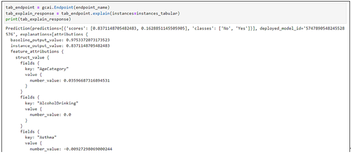
tab_endpoint = gcai.Endpoint(endpoint_name)
tab_explain_response = tab_endpoint.explain(instances=instances_tabular)
print(tab_explain_response)
Prediction results will be displayed as shown in the following figure which contains classes and the probability of the classes:

Figure 10.23: Predictions from deployed tabular classification model
Step 4: Explanations
Run the following lines of codes to get the explanations for the input record:
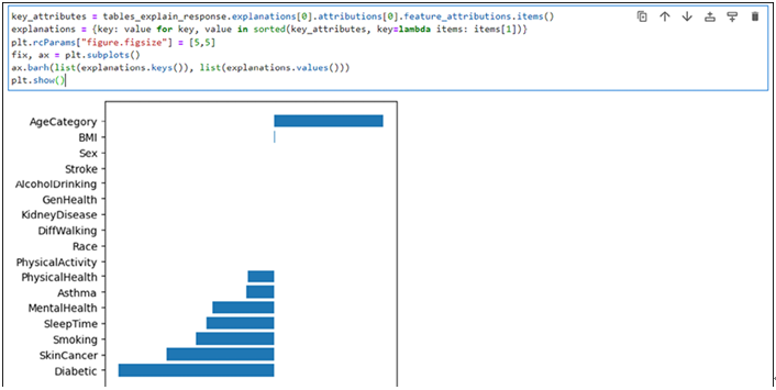
key_attributes = tables_explain_response.explanations[0].attributions[0].feature_attributions.items()
explanations = {key: value for key, value in sorted(key_attributes, key=lambda items: items[1])}
plt.rcParams[“figure.figsize”] = [5,5]
fix, ax = plt.subplots()
ax.barh(list(explanations.keys()), list(explanations.values()))
plt.show()

Shapley value is provided in the explanations for each of the features and it is visualized as shown in the following figure:

Figure 10.24: Explanations from deployed tabular classification model
Deletion of resources
We have utilized cloud storage to store the data, delete the files from the cloud storage manually. Dataset is created for image data and tabular data to delete them manually. Classification models for image and tabular are deployed to get the predictions and explanations, ensure to un-deploy the model from the endpoints and delete the endpoints (Refer Chapter 2, Introduction to Vertex AI & AutoML Tabular and Chapter 3, AutoML Image, text and pre-built models). Predictions are obtained using workbench, ensure to delete the workbench instance.

In case of the image data, users had to configure explainable AI during the training and deployment phase, whereas, in case of tabular data, explainable AI needs to be configured only during the deployment phase (AutoML will enable the explainable AI by default during the training phase for the tabular data). Follow the steps mentioned in Chapter 2, Introduction to Vertex AI & AutoML Tabular for the tabular dataset creation and tabular AutoML model training. Follow the below mentioned steps for the model deployment of the trained model.

Step 1: Trained model in the model registry

Trained model will be listed in the model registry as shown in the following figure:

Figure 10.17: Model registry (tabular classification model)

1. tabular_classification trained using AutoML. Click on the model and the version of the same.

Step 2: Deploy to end point

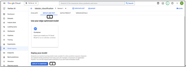
Once the model is selected (along with the version) users will get option to evaluate the model, deploy and test the model, and so on. Follow the steps mentioned below to deploy the model:

Figure 10.18: Trained tabular classification model

1. Select DEPLOY AND TEST tab.
2. Click DEPLOY TO ENDPOINT.

Step 3: Endpoint definition

Follow the steps mentioned below to define the endpoint:

Figure 10.19: Endpoint definition tabular classification model

1. Provide Endpoint name.
2. Click CONTINUE.

Step 4: Model settings

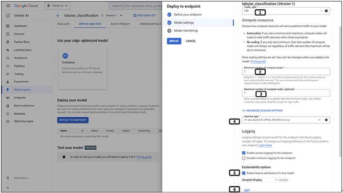
Follow the steps mentioned below to configure the model settings and to enable the explain ability options:

Figure 10.20: Model settings (enabling explain ability)

1. Set the Traffic split to 100.
2. Set the Minimum number of compute nodes to 1.
3. Set the Maximum number of compute nodes to 1.
4. Select n1-standard-8 in Machine type.
5. Enable the Explainability options.
6. Click EDIT.

Step 5: Set the Explainability options

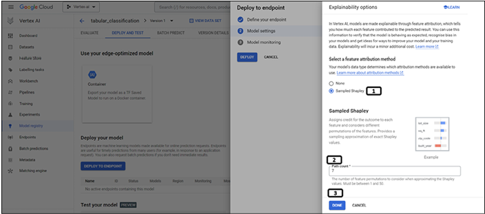
You can set the Explainability options by following the steps shown in the following figure:

Figure 10.21: Sampled Shapley path count

1. Select Sampled Shapley method.
2. Set the Path count to 7 (randomly chosen).
3. Click DONE.

Step 6: Model monitoring

Follow the below mentioned steps to disable the model monitoring (since it is not needed for the explanations):

Figure 10.22: Model monitoring

1. Disable Model monitoring options.
2. Click DEPLOY.

Once the model is deployed successfully, open the Jupyter lab from the workbench created and enter the Python code given in the following steps:
Step 1: Install the required packages
Type the following Python code to install the required packages:
!pip install tensorflow
!pip install pip install google-cloud-aiplatform==1.12.1

Step 2: Kernel restart
Type following commands in the next cell, to restart the kernel: (Users can restart kernel from the GUI as well):
import os
import IPython
if not os.getenv(“”):
Ipython.Application.instance().kernel.do_shutdown(True)

Step 3: Importing required packages
Once the kernel is restarted, run the following lines of codes to import the packages:
import base64
import tensorflow as tf
import google.cloud.aiplatform as gcai
import explainable_ai_sdk
import io
import matplotlib.image as mpimg
import matplotlib.pyplot as plt

Step 4: Input for prediction and explanation
Choose any image from the training set (stored in the cloud storage for the prediction) and provide the full path of the image chosen in the following code. Run the cell to read the image and covert the image to the required format:
img_input = tf.io.read_file(“gs://AutoML_image_data_exai/Kayak/adventure-clear-water-exercise-1836601.jpg”)
b64str = base64.b64encode(img_input.numpy()).decode(“utf-8”)
instances_image = [{“content”: b64str}]

Step 5: Selection of the endpoint select
Run the following lines of code to select the endpoint where the model is deployed. In this method, we are using the display name of the endpoint (instead of the endpoint ID). Image_ex is the endpoint name where the model is deployed. Full path of the endpoint (along with the endpoint ID) will be displayed in the output:
endpoint = gcai.Endpoint(gcai.Endpoint.list(
filter=f’display_name={“image_ex”}’,
order_by=’update_time’)[-1].gca_resource.name)
print(endpoint)

Step 6: Image prediction
Run the following lines of code to get the prediction from the deployed model:
prediction = endpoint.predict(instances=instances_image)
print(prediction)
Prediction results will be displayed as shown in the following figure which contains display names and the probability of the classes:

Figure 10.15: Image classification prediction result
Note: Since we are running this code using the Vertex AI workbench, we are not using service account for authentication.
Step 7: Explanations
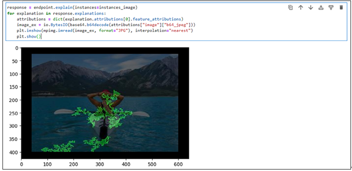
Run the following lines of codes to get the explanations for the input image:
response = endpoint.explain(instances=instances_image)

for explanation in response.explanations:
attributions = dict(explanation.attributions[0].feature_attributions)
image_ex = io.BytesIO(base64.b64decode(attributions[“image”][“b64_jpeg”]))
plt.imshow(mpimg.imread(image_ex, format=”JPG”), interpolation=”nearest”)
plt.show()

The output of the explanations is shown in the figure. Highlighted areas in green indicates areas/pixels which played important role for the prediction of the image:

Figure 10.16: Image classification model explanation

Once the model is trained, it needs to be deployed to end point for online predictions. Also create a workbench to get the predictions (python workbench will suffice). Follow the steps mentioned in the chapter Vertex AI workbench & custom model training., for creation of the workbench (Python workbench will suffice). Follow the below mentioned steps for the deployment of the models.

Step 1: Trained model listed under Model registry

Follow the below mentioned step to deploy the trained model:

Figure 10.10: Model registry

1. Click the trained model and then click on the version 1 of the model.

Step 2: Deploy to end point

Once the model is selected (along with the version) users will get the option to evaluate the model, deploy and test the model, and so on. Follow the steps mentioned below to deploy the model:

Figure 10.11: Image classification model deployment

1. Click DEPLOY AND TEST.
2. Click DEPLOY TO ENDPOINT.

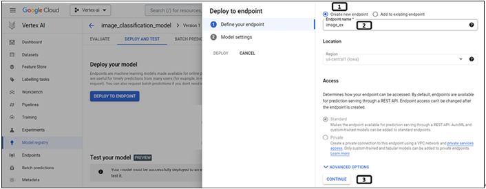
Step 3: Define end point

Follow the steps mentioned below to define the end point:

Figure 10.12: Image classification endpoint definition

1. Select Create new endpoint.
2. Provide the Endpoint name.
3. Click CONTINUE.

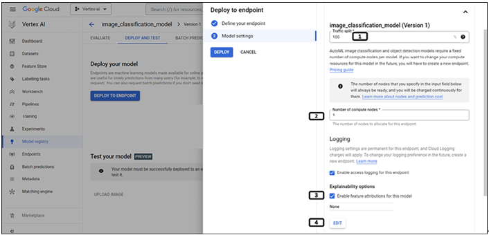
Step 4: Model settings

Follow the below mentioned steps to enable the explain ability of the model:

Figure 10.13: Image classification enabling explain ability

1. Set the Traffic split to 100.
2. Set the Number of compute nodes for predictions to be 1.
3. Enable the Explainability options.
4. Click EDIT.

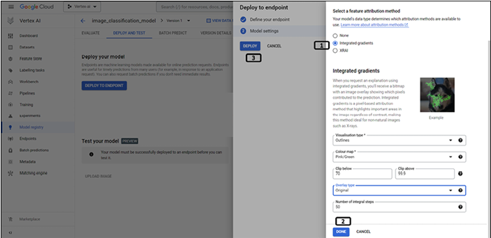
Step 5: Feature attribution method selection

Follow the below mentioned steps to set the feature attribution method selection. In this example we are using Integrated gradients method for the explanations:

Figure 10.14: Image classification explain ability configuration

1. Select Integrated gradients method for feature attribution method (Keep the values same for the all the parameters, what was set during the training phase).
2. Click DONE.
3. Click DEPLOY.

Check if the model is deployed properly and then proceed with the python code to get predictions and explanations.

Step 5: Explain ability

Explain ability needs to be set in two places while working on AutoML images. The first one is during the training phase of the model and while deploying the model. Follow the below mentioned steps to configure explain ability of the model during training phase.

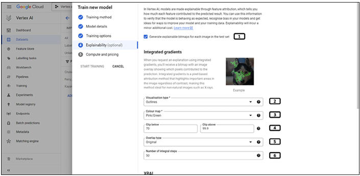
The steps shown below is for Integrated gradients method of Explainability as shown in the following screenshot:

Figure 10.7: Explain ability of image classification model

1. Enable to Generate explainable bitmaps.
2. Visualization type set to Outlines (pixels is another option to understand which pixels are playing important role for the prediction)..
3.  Color map select Pink/Green (Pink/Green color are used to highlight the areas on the image).
4.  Clip below and Clip above parameters are used to reduce the noise. Enter 70 and 99.9 for click below and above respectively.
5. Select Original under Overlay type (pixels will be highlighted on top of the original image).
6. Enter 50 for the Number of integral steps (increasing this parameter will reduce the approximation error).

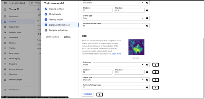
Scroll down and follow the steps mentioned in the following step to set the parameters for XRAI method:

Figure 10.8: Explain ability of image classification model (XRAI)

1. Choose the Color map.
2. Clip below and Clip above parameters are used to reduce the noise. Enter 70 and 99.9 for click below and above respectively.
3. Select Original under Overlay type (pixels will be highlighted on top of the original image).
4. Enter 50 for the Number of Integral steps (increasing this parameter will reduce the approximation error).
5. Click CONTINUE.

Step 6: Compute and pricing

Follow the below mentioned steps to configure the budget for the model training:

Figure 10.9: Compute and training for image classification model

1. Set the minimum node hours for 8 (it is the minimum value for image data).
2. Click START TRAINING.

It will take a few hours to train the image classification model. Prediction and the explanation for the prediction can be obtained.

In this exercise, we will try to understand how explainable AI can be used to understand model prediction using image data and the tabular data with the help of AutoML of Vertex AI. The data used for AutoML tables and images will be used for this exercise as well. (Refer chapters Introduction to Vertex AI and AutoML Tabular and AutoML Image, text and pre-built models).

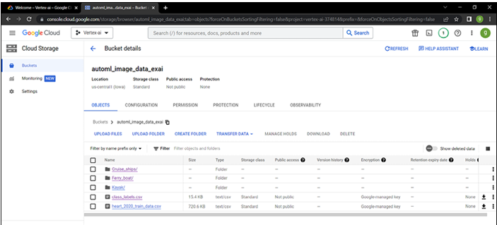
AutoML_image_data_exai bucket is created under us-centra1 (single region).

Three folders containing image data (Cise_ships, Ferry_boat and Kayak) is uploaded and CSV file (class_labels.csv) is created as shown in Chapter 3, AutoML Image, text and pre-built models (refer Figure 3.1 and 3.2 for csv creation). heart_2020_train_data.csv is uploaded to the same folder which will be used for AutoML tables. Figure 10.2 shows the data uploaded to the cloud storage:

Figure 10.2: Data uploaded to the cloud storage

Model training for image data

The initial steps for dataset creation for the image data will have no changes. Refer Image dataset creation of Chapter 3, AutoML Image, text and pre-built models and follow the below mentioned steps for AutoML model training.

Step 1: Train new model

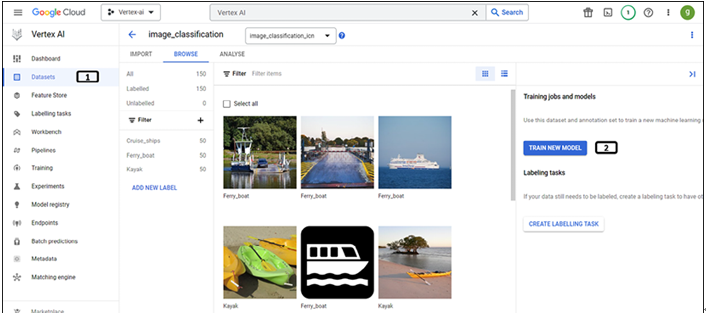
Newly created dataset will be listed under the dataset of the Vertex AI. Follow the below steps to initiate the model training as shown in the following screenshot:

Figure 10.3: Image dataset created on Vertex AI

1. Click on Datasets section of Vertex AI (open the newly created image dataset).
2. Click TRAIN NEW MODEL.

Step 2: Training method selection

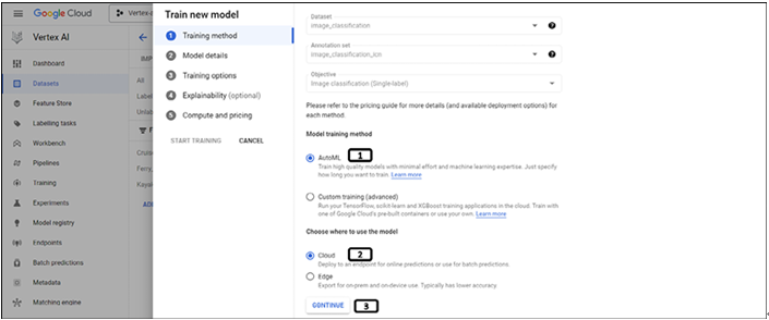
Training method step does not have difference as mentioned in Chapter 3, AutoML Image, text and pre-built models. Follow these steps to set the training method:

Figure 10.4: Training method selection

1. Select AutoML.
2. Select Cloud (we will deploy the model to get predictions and explanations).
3. Click on CONTINUE.

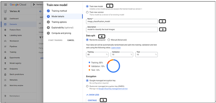
Step 3: Model details

Follow the steps mentioned below to set the model details:

Figure 10.5: Image classification model details

1. Select Train new model.
2. Provide a Name for the model.
3. Provide Description for the model.
4. Under Data split select Randomly assigned.
5. Click CONTINUE.

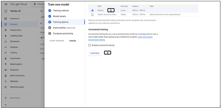
Step 4: Training options

Follow the below mentioned steps for training options:

Figure 10.6: Image classification training options

1. Select Default training method.
2. Click CONTINUE (we do not have to enable incremental training for the explainable AI).

Each approach for attributing features is based on Shapley values, which is an algorithm derived from cooperative game theory that gives credit for a given result to each participant in a game. When this concept is applied to models for machine learning, it indicates that each model feature is dealt with as if it were a “player” in the game. The Vertex Explainable AI provides a certain amount of credit to each individual characteristic based on its weight in the overall forecast:

• Sampled Shapley method: The sampled Shapley technique offers an estimate of the actual Shapley values via the use of sampling. Tabular models created using AutoML make use of the sampled Shapley approach to determine the relevance of features. For these models, which are meta-ensembles of tree and neural network structures, the Sampled Shapley method performs quite well.
• Integrated gradients method: Along an integral route, the integrated gradients approach calculates the gradient of the prediction output with respect to the characteristics of the input. This is done to get an accurate result. Calculations of the gradients are performed at various time intervals along a scaling parameter. Utilizing the Gaussian quadrature rule allows for the calculation of the size of each interval. (When dealing with picture data, think of this scaling option as a “slider” that sets all the image’s pixels to a black value.) The integration of the gradients is done as follows:
  • An approximation of the integral may be found by using a weighted average.
  • Calculations are performed to get the element-wise product of the original input and the averaged gradients.
• XRAI method: To discover which parts of a picture that contribute the most to a certain prediction of class, the XRAI approach uses a combination of the integrated gradients method and some extra phases.
• Pixel-level attribution: XRAI can do pixel-level attribution for the picture that is sent into it. In this stage of the process, XRAI makes use of the integrated gradients approach, applying it to both, a black and a white baseline.
• Over segmentation: XRAI generates a tiny patch over the picture by over segmentation , which is done independently of pixel-level attribution. In order to construct the picture segments, XRAI takes advantage of Felzenswalb’s graph-based technique.
• Region selection: XRAI compiles the pixel-level attribution included inside each segment to calculate the attribution density of that segment. XRAI assigns a ranking to each segment based on these values, and then it arranges the segments from most positive to least positive. This identifies which parts of the picture contribute the most strongly to a certain class prediction, as well as which parts of the image are most prominent.

All types of models are supported for feature-based explanations. Classification models are supported for AutoML images and classification, and regression models are supported for AutoML tabular models.

In the case of explanations based on examples, Vertex AI makes use of the closest neighbor search to produce a list of instances (usually taken from the training set) that are most comparable to the input. These examples allow users to investigate and clarify the behavior of the model since users can reasonably anticipate that comparable inputs would result in similar predictions.

Consider the following scenario: users have a model that analyzes photos to determine whether they depict a bird or an aircraft; however, the model incorrectly identifies certain birds as planes. To figure out what is going on, we may extract other photos from the training set that is comparable to the one we are looking at and utilize example-based explanations to explain what is occurring. When we look at those instances, we see that many of the incorrectly identified birds and the training examples that are comparable to them are dark silhouettes and that most of the dark silhouettes that were aircraft were found in the training set. This suggests that users might potentially increase the quality of the model by including more silhouetted birds in the training set.

Explanations that are based on examples may also help identify confusing inputs that might be improved with human labelling. Models that provide embedding or latent representation for input variables are supported. Tree based models which do not provide embeddings for the inputs are not supported in examples-based explanations.

Feature-based explanations

Feature-based explanations is another way of explaining model output based on the features. The amount of contribution that each feature in the model made to the predictions that were made for a particular instance is shown by the feature attributions. When users make a request for predictions, they will get anticipated values that are suitable for the model you are using. Feature attribution info will be provided when users request for the explanations.

Feature attributions work on image and tabular data. They are supported for AutoML and custom trained models. (Classification models only for image data and classification/regression models for tabular data).

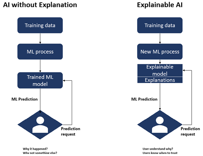
Artificial intelligence has the ability to automate judgments, and the outcomes of such decisions may have both beneficial and bad effects on businesses. It is essential to have an understanding of how AI comes to its conclusions, just as it is essential to have this understanding when recruiting decision is made for the business. A great number of companies are interested in using AI, but are hesitant to hand over decision-making authority to the model or AI simply because they do not yet trust the model. Explainability is beneficial in this regard since it offers insights into the decision-making process that models use. Explainable AI is a crucial component in the process of applying ethics to the usage of AI in business. Explainable AI is predicated on the notion that AI-based applications and technology should not be opaque “black box” models that are incomprehensible to regular people. Figure 10.1 shows the difference between AI and Explainable AI:

Figure 10.1: Explainable AI

In the majority of the scenarios developing complex models is far easier than convincing stakeholders that the model is capable of producing decisions that are superior to those produced by humans. It is not the same thing as having greater accuracy scores or a lower RMSE to make a better judgment. A correct conclusion may be reached by providing accurate data as input. In many cases, the person making the choice is the one who needs to comprehend it. For them to feel at ease handing over the decision-making to the model, they need to understand how the model came to its conclusions.

Explainable AI is essential to the development of responsible AI because it offers an adequate amount of transparency and responsibility for the choices made by complicated AI systems. This is of utmost importance when it comes to artificial intelligence systems that have a substantial influence on the lives of people.

XAI on Vertex AI

Explainable AI of Vertex AI provides explanations that are either feature-based or example-based in order to give a better understanding of how models make decisions. Anyone who builds or uses machine learning will gain new abilities if they learn how a model behaves and how it is influenced by its training dataset. These new abilities will allow users to improve their models, increase their confidence in their predictions, and understand when and why things work.